![]()


Water-Distribution System Modeling as a Tool to Assist Epidemiologic Investigations at Dover Township, New Jersey
Morris L. Maslia, M. Jason B. Sautner, Mustafa M. Aral, Juan J. Reyes, John E. Abraham, and Robert C. Williams
ABSTRACT
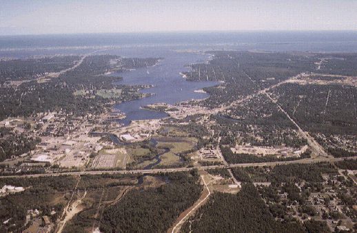
Toms River Areal View
An epidemiologic study of childhood leukemia and central nervous system cancers that occurred in the period 1979 through 1996 in Dover Township, New Jersey, is being conducted. Because groundwater contamination has been documented historically in public- and private-supply wells, there is the possibility of exposure through this pathway. The Dover Township area has been primarily served by public water supply that relies solely on groundwater; therefore, a protocol has been developed for using a water-distribution model such as EPANET as a tool to assist the exposure assessment component of epidemiologic investigation. The model is being used to investigate the question of human exposure to groundwater contaminants. Because of the unavailability of historical data, the model was calibrated to the present-day (1998) water-distribution system characteristics. Pressure data were gathered simultaneously at 25 hydrants throughout the distribution system using continuous recording pressure data loggers during 48-hour tests in March and August 1998. Data for storage tank water-levels, system demand, and pump and well status (on/off) were also obtained. Field-data gathering procedures, calibration results and water-quality simulation using a naturally occurring element (barium), as well as an analysis indicating the percent of water originating from points of entry to the water-distribution system for 1998 conditions are presented.
On Toms River
INTRODUCTION
In January 1997, the Agency for Toxic Substances and Disease Registry (ATSDR) was requested to assist with a case-control epidemiologic investigation, being conducted by the New Jersey Department of Health and Senior Services (NJDHSS), of childhood leukemia and central nervous system cancers that occurred in the period 1979 through 1996 (Berry and Haltmeier, 1997) in the Dover Township area (Figure 1). Epidemiologic research generally employs non-experimental (observational) studies in which exposure is not assigned or controlled by the investigator, owing to ethical issues associated with experimental studies. There are two types of observational study designs that are most commonly used in epidemiologic investigations: cohort and case-control studies. In a case-control study, a population is delineated and cases of disease arising in that population over a specified time period are identified. The exposure experiences of the case group are compared to the exposure experiences of a sample of the non-diseased persons in the population from which the cases arose (Rothman and Greenland, 1998). A case-control design is an efficient method for studying risk factors for rare diseases such as childhood cancers. For the case-control study being conducted by the NJDHSS, environmental exposures that are more common in cases (cases are children diagnosed with certain cancers) may be considered as possible risk factors for disease (such as childhood leukemia and brain and central nervous system cancers). One risk factor being considered by ATSDR and NJDHSS is the potential for exposure to contaminated potable water.
There have been previous investigations trying to relate water-supply contamination with health effects. Lagakos et al. (1986) describe an association between exposure to trichloroethylene-contaminated drinking water and increased prevalences of stillbirths and central nervous system defects, oral defects, and chromosomal defects. To investigate the potential reproductive health effects of long-term, low-dose exposure to waterborne chloroform, Kramer et al. (1992) conducted population-based case control analyses to study the association of trihalomethanes with low birth-weight, prematurity, and intrauterine growth retardation using state of Iowa birth certificate data. Bove et al. (1995) used environmental and birth outcome databases for a four-county area in northern New Jersey to study the effects of public drinking water contamination on birth outcomes.
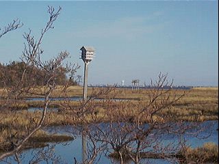
Toms River Marsh Area
Ideally, to conduct their investigation, the NJDHSS would have liked for ATSDR to establish the concentration of water at the tap that a household might have received. However, this task was not possible given the paucity of contaminant-specific concentration data during the desired study time frame. As an alternative, scientists from the NJDHSS would like information on the percentage of water that a person might have received during the study period from points of entry to the water-distribution system serving the residents of the Dover Township area (Figure 1). This would allow the investigators to assess the association of the occurrence of childhood cancer with exposure to each of the sources of potable water entering the distribution system, including ones known to be historically contaminated.
EXPOSURE ASSESSMENT APPROACH
Groundwater contamination of water-supply wells in Dover Township has generally consisted of volatile organic compounds (VOCs) such as trichloroethylene (TCE) and semi-volatile organic compounds (SVOCs) such as styrene-acrylonitrile (SAN) trimer (NJDHSS, 1999c). The reader is referred to the following reports for a description and analysis of the contamination of groundwater resources: ATSDR (1988, 1989), Malcolm Pirnie, Inc. (1992), Pinder, et al. (1992), and NJDHSS (1999a, b, c). Groundwater is the source of potable water in the area and approximately 85 percent of the current Dover Township area residents are served by a public-supply system. Therefore, there exists the possibility of human exposure to these contaminants through the groundwater pathway and an analysis of the potential for distribution of contaminants through the water-distribution system was deemed necessary.
In a distribution system such as the one serving the residents of the Dover Township area, not all public-supply wells may become contaminated. Furthermore, some supply wells affect certain areas more than other wells, and disease cases may have no relationship with contaminant sources. Therefore, we will be using the concept of "proportionate contribution" to assess the contribution of water from various points of entry of the distribution system to subject residences. Because the focus of the epidemiologic investigation is on children, exposure at residential locations is deemed as the most important exposure source to investigate, although other exposure sources may be present. Based on residence histories, reconstruction of historical water-distribution system characteristics can be used to estimate exposure to specific water sources by determining the percent of water study subjects may have received from each of the points of entry to the water-distribution system.
It is important to note that the analysis of the water-distribution that we have undertaken, the proportionate contribution of different water sources to the supply for cases and controls, is but merely one component of an overall exposure assessment being conducted by the NJDHSS to address issues of concern to the community. Other aspects that are being addressed include obtaining valid residential histories, estimating consumption patterns, conducting a study based on data gathered from birth certificates, and the possibility of exposure to contaminants from other environmental media such as air and soil.
To address a particular issue of concern to the community, assist the NJDHSS, and reconstruct historical water-distribution system characteristics, we have chosen to use a water-distribution system model. The use of water-distribution system modeling for estimating exposure has been described in the literature by several investigators. Murphy (1986) calculated exposure to TCE from Wells G and H in Woburn, Massachusetts by using a water-distribution model to assess various pumping and water-use configuration patterns during each month that the wells were in operation. Clark et al. (1991) and Geldreich et al. (1992) used extended period simulation hydraulic and dynamic water-quality models to investigate the distribution of occurrences of illness due to waterborne contaminants (escherichia coli sterotype 0157:H7) found in the Cabool, Missouri, distribution system. Clark et al. (1996a, b) used the EPANET water-distribution system model to develop several scenarios to explain possible pathogen transport of waterborne Salmonella typhimurium outbreak in the Gideon, Missouri, municipal water system. Aral et al. (1996) and Aral and Maslia (1997) used the EPANET water-distribution system model in conjunction with a geographic information system (GIS) to simulate four exposure scenarios for the Southington, Connecticut, water-supply system that used groundwater contaminated with VOCs during the 1970s. For our evaluation, the EPANET water-distribution model, integrated with spatial analysis technologies, is being used to model the water-distribution system serving the residents of the Dover Township area.
In this paper, we present three aspects of the exposure assessment effort that will use a model for historical reconstruction of the hydraulic characteristics of the water-distribution system. These aspects are: (1) the field-data gathering procedures, (2) model calibration results and water-quality simulation, and (3) simulations that have been conducted on the present-day system to estimate the percent of water originating from each of eight points of entry to various locations throughout the water-distribution system.
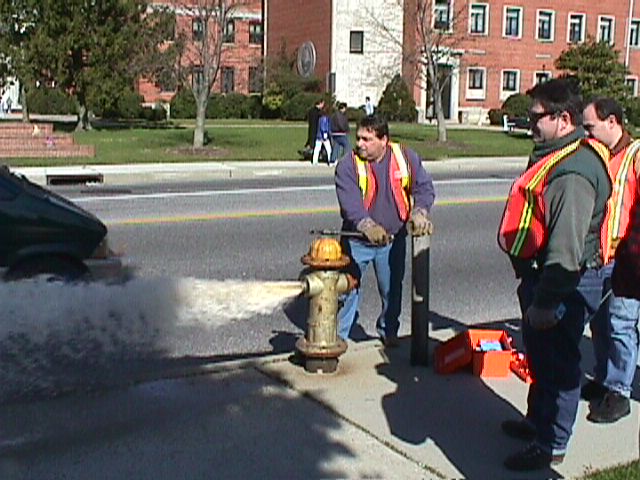
Toms River Hydrant Testing
DESCRIPTION OF THE WATER-DISTRIBUTION SYSTEM
The water-distribution system being investigated has been operating since 1897. It serves the residents of Dover Township, New Jersey, including the Toms River area, and communities outside of Dover Township including the borough of South Toms River and a portion of Berkeley Township (Figure 1). At the end of 1997, the water-distribution system served a population of 92,160 persons that consisted of 44,510 customers. The distribution system consists of 785.7 km (488.2 mi) of mains, ranging from 40.6 to 5.1 cm (16 to 2 in.) in diameter, three elevated and six ground-level storage tanks with a total rated storage volume of 2.78x10⁷ L (7.35 Mgal), 23 groundwater extraction wells in eight well fields with a combined rated capacity of 1.02x10⁸ L/d (27 Mgal/d), and 17 high service or booster pumps (Board of Public Utilities, 1997). Water from seven of these wells is pumped directly into the distribution system (e.g., wells 20, 31), whereas the remaining 16 wells are used to fill storage tanks (e.g., well 40 and the Windsor ground-level storage tank) and then high service or booster pumps are used to supply the distribution system with water from the storage tanks (Figure 1).
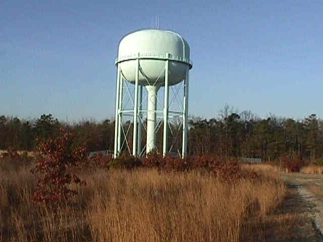
Elevated Storage Tank
Demand for water in the Dover Township area is characterized by two typical demand patterns. A winter-time demand pattern, typical of data collected in March 1998 (Figure 2A), generally occurs from October through mid-May of the year. In March 1998, based on field observations (Sautner and Maslia, 1998), demand was equal to 2.9x10⁷ L/d (7.6 Mgal/d). Peak-demand conditions, typical of field data collected in August 1998 (Figure 2B) and equal to 6.1x10⁷ L/d (16.1 Mgal/d), generally occur during the summer season from the end of May (Memorial Day) through September of the year (Maslia and Sautner, 1998b). Thus, the average annual demand based on 1998 field data is approximately 4.5x10⁷ L/d (12 Mgal/d).
COLLECTION OF FIELD DATA
There were primarily two reasons for developing a protocol for a synoptic, system-wide collection of hydraulic and operational data. First, to understand the present-day distribution of water from points of entry (sources) to locations throughout the distribution system, a calibrated model of the distribution system needed to be developed; however, a database of spatially and temporally varying data by which to characterize the distribution system was not available. Second, to reconstruct historical characteristics of the water-distribution system, a synoptic, system-wide characterization of the water-distribution system, based on measured data was required. Neither present-day or historical system-wide pressure measurements were available for the water-distribution system being investigated. Hence, investigators decided to obtain present-day measurements in order to accurately characterize the water-distribution system.
ATSDR investigators, in coordination with the NJDHSS and the water utility operators, developed a protocol to collect pressure data and operational information during winter- and peak-demand periods of the year–March and August 1998, respectively. Details of the protocol are provided in Maslia and Sautner (1998a) and are briefly described below.
Hydrant Selection
Twenty-five hydrants (out of a system total in 1997 of 2,127) were initially selected as test hydrants (designated as H-1, H-2, etc.) on which continuous pressure recording equipment would be installed. The number and locations of the test hydrants (H-1, H-2, etc., shown in Figure 1) were selected based on the following considerations:
Initial simulations conducted with EPANET indicated areas of questionable high pressure (exceeding 862 kPa (125 psi)) within the water-distribution system. The data used as input for the simulations were supplied by the water-utility. According to water-utility staff, the data represented an equivalent hydraulic network of 15.2 cm (6 in.) and larger diameter pipelines for 1993 conditions (Flegal, 1997). Therefore, hydrant locations were selected to assist in determining the actual pressures that exist in these areas.
Hydrant locations were also selected to provide as complete as possible a system-wide coverage so that effects from storage tank and pump operations could be characterized by pressure changes at these hydrants.
ATSDR used additional hydrants for quality assurance purposes in the event that data collection devices failed to operate properly, or that hydrants became inoperable or unusable during the test.
ATSDR responds to and tries to accommodate stakeholder input when conducting site activities. In the case of modeling the water-distribution system serving Dover Township, area residents wanted assurances that a sufficient number of measuring locations would be available to accurately characterize the distribution system. Because ATSDR scientists determined that additional data-collection locations would not abrogate the scientific merits of the field test, additional monitoring locations requested by area residents were also included.
As part of a quality assurance program, 25 hydrants were selected as alternate test hydrants (designated as AH-1, AH-2, etc.) in the event that any of the original 25 test hydrants could not be used to monitor pressure during the test periods. During the installation of the data gathering equipment on the hydrants, it was determined that 5 of the designated test hydrants (H-5, H-6, H-14, H-19, and H-22) were not suitable for use as measuring points. Therefore, the associated alternate hydrants (AH-5, AH-6, AH-14, AH-19, and AH-22) were used. The final set of test hydrants used for both the March and August 1998 tests is shown in Figure 1. These 25 hydrants are connected to network pipelines that: (1) were installed between 1963 and 1996, (2) are constructed of asbestos cement (14 hydrants), plastic (PVC, 10 hydrants), and ductile iron (1 hydrant) materials, and (3) range in diameter size from 30.5 to 15.2 cm (12 to 6 in.).
Data Recording Equipment
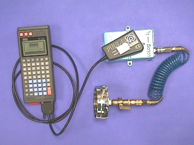
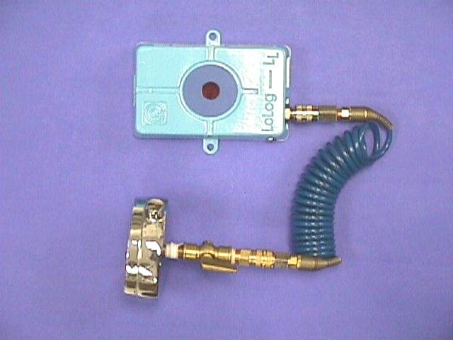
RADCOM Lolog LL(TM)
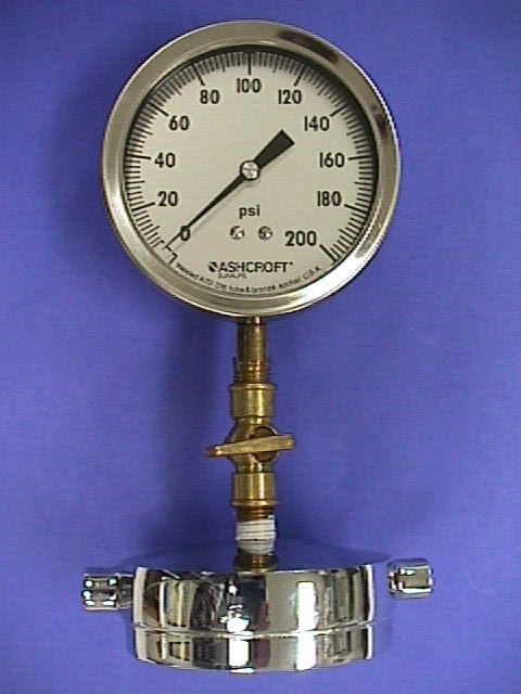
Pressure Gage
Each test hydrant was equipped with a RADCOM Lolog LL™ continuous pressure data logger that sampled pressures at 1-minute intervals. The intent of the test was to collect time-series pressure data over a 48-hour test period. At the conclusion of the test, data from each logger was downloaded to a Psion HC-120™ hand-held computer for storage and post-test analysis.
Test Protocol
A test protocol was developed by ATSDR to insure that successful data-gathering would occur during field-test activities and to establish quality assurance procedures that would be followed for each hydrant to be monitored (Maslia and Sautner, 1998a). Prior to conducting the tests, the loggers were factory calibrated to 1034 kPa (150 psi). The following procedure was used to install and quality-assure the installation on each of the 25 hydrants for the March and August 1998 field tests:
A hydrant was opened and flushed to remove debris; when clear running water was observed, the hydrant was shut off.
A hydrant adapter kit, brass shut-off valve, and pressure gauge were installed on the hydrant.
The hydrant was reopened, and a pressure reading was obtained from the pressure gauge and recorded in a log book. At this point, a check was made for any leaks occurring around the pressure gauge connection and the hydrant adapter kit.
The pressure gauge was removed and the RADCOM Lolog LL pressure data logger was now attached to the hydrant and hydrant adapter kit, and a check was made for any leaks occurring around the pressure data-logger connection and the hydrant adapter kit. A pressure reading was obtained from the logger and compared with the gauge pressure recorded earlier.
ATSDR staff in the water utility’s operations control room recorded the operational history of wells and booster pumps for the duration of the tests. They also manually recorded instantaneous system production data and storage tank water levels being recorded electronically by the water utility’s supervisory control and data acquisition (SCADA) system.
Throughout the tests, ATSDR and NJDHSS staff periodically checked each test hydrant and pressure data logger to assure that the logger was functioning properly and that water leaks, potentially affecting the pressure measurements, had not developed. After the test was concluded, the loggers were removed by reversing the process described in steps 1-4 above, and the data was downloaded to and stored in the hand-held Psion HC-120™ computer. Analysis of pressure data from both tests indicate that throughout the water-distribution system pressures generally range from a low of 276 kPa (40 psi) to a maximum of slightly more than 689 kPa (100 psi). Details of the tests are provided in reports by Sautner and Maslia (1998) and Maslia and Sautner (1998b).
WATER-DISTRIBUTION SYSTEM MODEL DEVELOPMENT
Historical Background
Using mathematical models to analyze flow in water-distribution system networks has been in existence for more than 60 years since it was proposed by Cross (1936) in the 1930s. Hydraulic models can be used to analyze systems where demand and operating conditions are static or are time varying. The former is a ‘steady-state’ model, and the latter is referred to as an ‘extended period simulation’ (EPS) model.
Modeling the spatial distribution of water quality in pipelines first began with a steady-state modeling approach suggested by Wood (1980) who studied slurry flow. The representation of temporally varying conditions for contaminant movement in a distribution system or ‘dynamic’ water-quality models began to be used in the mid-1980s. With the widespread use and relatively low cost of personal computers and desktop workstations during the mid-1980s and 1990s, there are now many models, both proprietary and public domain, that can be used to conduct hydraulic and water-quality analyses. The reader is referred to Rossman (1999) and Clark (1999) for a thorough discussion on the development and evolution of hydraulic and water-quality models.
Hydraulic and Water-Quality Simulation Model
Hydraulic modeling of water-distribution systems can be conducted by solving mathematical equations that describe the pipe network of the distribution system. Extended period simulation represents a succession of steady-state solutions as demands and tank levels change over fixed points in time. For each point in time, at network nodes (junctions), an equation for conservation of mass is solved. At each network pipe (link), an equation relating head loss and flow is solved. The mathematical equations for the development of the hydraulic simulation model and the numerical methods used to solve the equations are referenced in the published literature, and because of space limitations, will not be given here. For details, the reader should refer to Rossman (1994), Rossman et al. (1994), Todini and Pilati (1987), and Salgado et al. (1988).
The fate of a dissolved substance flowing through a distribution network over time is tracked by EPANET’s dynamic water quality simulator. To model water quality of a distribution system, EPANET uses flow information computed from the hydraulic simulation as input to the water-quality model. The water quality model uses the computed flows to solve the equation for conservation of mass for a substance within each link. The equations used to describe the fate and transport of a substance flowing through a distribution network by EPANET and the numerical method used to solve the equations are described in Rossman (1994) and Rossman et al. (1993, 1994).
The identification of the source of delivered water in a distribution system has become a necessity when attempting to determine the location of a source that may supply water that exceeds a given level of a chemical or biological constituent. Wood and Ormsbee (1989) developed an explicit method to calculate the percentage of flow originating at various source points at a specific location in a distribution system. EPANET also has the ability to track the percent of water reaching any point in the distribution network over time from a specified location (source) in the network. Given the multiple number of points of entry to the water-distribution system serving the residents of Dover Township, the ability to track the percent of water originating from a point of entry becomes a very useful analysis tool for our investigation.
HYDRAULIC MODEL CALIBRATION
Overview
With a computer model of the water-distribution system, we are trying to reproduce the behavior of a real hydraulic system as closely as possible in terms of spatial and temporal characteristics. The collection of field data provides an opportunity to understand the operation of the real system at a specified number of locations and times. Such efforts are consistent with the American Water Works Association Engineering Computer Applications Committee who find that "true model calibration is achieved by adjusting whatever parameter values need adjusting until a reasonable agreement is achieved between model-predicted behavior and actual field behavior (AWWA Engineering Computer Applications Committee, 1999)." Once a model is considered to be calibrated, it can then be used to, among other purposes, estimate hydraulic characteristics of the real system at locations where measured data are unavailable or unknown, spatially and temporally.
According to the AWWA Engineering Computer Applications Committee (1999) there are 10 sources for possible error that could cause poor agreement between simulated model values and measured field values. These sources of error provide a potential list of parameter values that can be adjusted during the model calibration process and are: (1) errors in input data (measurement and typographical), (2) unknown pipe roughness values (i.e., Hazen-Williams "C-Factors"), (3) effects of system demands (distributing consumption along a pipe to a single node), (4) errors in data derived from network maps, (5) node elevation errors, (6) errors introduced by time variance of parameter values such as tank water levels and pressures, (7) errors introduced by a skeletal representation of the network as opposed to modeling all small-diameter pipes, (8) errors introduced by geometric anomalies or partially closed valves, (9) outdated or unknown pump-characteristic curves, and (10) poorly calibrated measuring equipment including data loggers, tank water-level monitors, and SCADA systems. Owing to brevity and space limitations, it is not feasible, in this paper, to discuss each of these sources of error with respect to the data obtained for the distribution system under consideration. However, after careful review of the data and the possible sources of error, investigators narrowed the list to three parameters that are believed provide the greatest source for error for our situation and therefore, subjected to possible adjustment during the calibration process. The parameters are: (1) pipe roughness values (Hazen-Williams "C-Factors"), (2) system demand factors, and (3) pump-characteristic curves (head versus flow values). A detailed discussion of values assigned to these parameters and adjustments made during the model calibration process is provided below in the section on "Calibration Parameters ."
Data Sources and Calibration Methodology
Physical characteristics of the distribution system (pipe, pump, storage tank, and well data) were obtained from databases supplied by the water utility (Flegal, 1997). Sources for the data and model parameter values are listed in Table 1. Based on the information supplied by water utility, ATSDR developed a model network consisting of 16,071 pipeline segments (links) and 14,987 junctions (nodes). Table 2 describes the material type for pipes composing the network as of the end of 1997, and as shown, most of the network is composed of asbestos cement and plastic (PVC) pipes. Because the goal of our investigation is to conduct a population-based assessment, geo-spatial location information for network facilities was required. Therefore, geographic coordinates for the network nodes were determined by using global positioning system (GPS) equipment to obtain locations of the 50 test and alternate hydrants, wells, and storage tanks, in conjunction with TIGER/Line™ files (1992) for the Dover Township area. In addition to spatial coordinates, land surface elevation values for the measuring points (hydrants) were also obtained by using GPS equipment. Elevation values for network nodes were obtained from 7.5-minute U.S. Geological Survey Digital Elevation Model quadrangles for the Dover Township area and assigned to network nodes by using GIS software.
The model was calibrated to the hydraulic and operational data collected during the March 1998 test and then confirmed against data collected during the August 1998 test. The model was run as an EPS using one-hour hydraulic time steps and demand-pattern factors derived from the control-room data collected during the tests (Figure 2a and Figure 2b). Consumption data required by the model at nodal locations throughout the distribution service area were based on metered billing records collected quarterly by the water utility, from October 1997 through April 1998. The consumption data were allocated by using an address-matching technique and GIS software to locate the water meter address to the nearest model node.
In order to accommodate the hourly-time step pattern of the EPS required by EPANET, the one-minute sampling data that were collected during the field tests were averaged to one-hour time periods. Hourly pressure data, based on the one-minute sampling data for 5 of the 25 test hydrants are shown in Figure 3 for the March and August 1998 tests. Because of space limitations, it is not possible to show data and results for all 25 test hydrants in this paper. However, it is important to note that the model calibration analyses and results are based on simulations from all 25 hydrants. Therefore, further discussion of simulation results will focus on the 5 hydrants that represent the southwest (test hydrant H-1), south-central (test hydrant H-11), central (test hydrant H-17), northwest (test hydrant H-20), and northeast (test hydrant AH-22) portions of the study area (Figure 1).
To simulate groundwater wells pumping directly into the distribution system or into storage tanks, well-flow data from the SCADA system was recorded by ATSDR staff during the tests. For model calibration purposes, flow from multiple wells in a well field to a tank, such as Parkway well field or Holly Plant well field (Figure 1), was combined and assumed to be one well. The well (or combined wells for a well field) was associated with a model junction and a negative base demand was assigned to the junction, indicating inflow to the network or to a tank. Because EPANET allows one to assign a different demand pattern to each junction in the model, each well or well field was assigned a demand pattern based on the recorded SCADA-system data. These demand patterns were used to simulate varying flow rates and the on/off cycling of the wells during the test.
Comparisons of measured pressure with simulated pressure for the March and August 1998 tests at the 5 test hydrants are presented in Figure 3. Comparisons between measured and simulated hydraulic heads are presented in Figures 4A and 4B. (Measured hydraulic heads were derived from measured water levels in the tanks and the elevation of the bottom of the tanks.) Comparison of measured and simulated pump flows are presented in Figure 5. Described below are the model parameters that were adjusted for the calibration process and analysis of the results of the March and August 1998 simulations.
Calibration Parameters
Three model parameters were considered for variation with respect to model calibration: (1) pipe roughness (Hazen-Williams "C-Factor"), (2) system demand factors, and (3) pump-characteristic curves (head versus flow values). Discussions with the water utility staff revealed that the network pipes had very little scaling or deposition, and inspections have shown very little debris. Additionally, as shown in Table 2, more than one-third of the pipes (in quantity and lengthwise) are made of PVC where the variation in "C" is negligible. Therefore, initial estimates for "C", obtained from published tabular values (Rossman, 1994) and listed in Table 2 for every pipe material type, were not varied during the calibration process. Subsequent to model calibration, a sensitivity analysis confirmed that for our investigation, variation in "C-Factor" has an insignificant influence on system pressures and flow directions.
Initial estimates of system demand factors were obtained by ATSDR staff recording production data during the tests from the control-room SCADA-system output. In EPANET, the system demand factors are used to distribute the average daily nodal consumption values over hourly time steps of an EPS. Therefore, for the March and August 1998 tests, the system demand factors distributed the average nodal consumption values over the 48 hourly time steps of the EPS that were used to model the field tests. During the calibration process, the individual hourly factors were modified. The factoied by a trial and error method using the generalized diurnal pattern shown in Figures 2a and 2b as guidance for adjusting the factors (e.g., peak demand occurring at approximately 0800 and 1900 hours; low demand occurring at approximately 0300 and 1600 hours). Factors for the August test were modified from factors for the March test because the conditions of each test represented different demand conditions–winter-time demand for the March test and peak demand for the August test. It is important to note, however, that although individual hourly factors were modified, the total system-wide demand, 2.9x10⁷L/d (7.6 Mgal/d) for March and 6.1x10⁷ L/d (16.1 Mgal/d) for August was not modified during the calibration process. The calibrated values for the hourly demand factors for the March and August 1998 test are shown in Figures 2a and 2b.
Consumption data are needed as input for EPANET at nodal locations throughout the model network that represents the distribution system service area. These data were provided by the water utility and represented metered billing records collected quarterly from October 1997 through April 1998. The consumption data were distributed to model nodes by using an address-matching technique and GIS software to assign the water meter address to the adjacent (and nearest) model node. If more than one meter address was adjacent to a model node, then the consumption for the node was the sum of all metered consumption adjacent to the node. Because our model is composed of pipes as small as 5-cm (2-in.) in diameter, the density of the model network is such (14,987 nodes) that errors due to incorrect or inaccurate distribution of consumption are minimal and insignificant. Therefore, the spatial (nodal) distribution of consumption in terms of an average daily value derived from records provided by the water utility, was not modified during the calibration process. Rather, as discussed above, the system demand factor pattern in EPANET was used to distribute the average daily consumption value to an hourly time step value.
A third model parameter that was adjusted during the calibration process was the high service and booster pump-characteristic curves. Initial pump-characteristic curve data were provided to ATSDR by the water utility (Flegal, 1997), and these are listed in Table 3. However, the source of the data (manufacturer’s data, field testing, etc.) was unknown. Therefore, this was a key parameter that could justifiably be modified during the calibration process. Modifications were made to the original data so that system operations, as observed during the two tests, could be duplicated as closely as possible. The calibrated pump-characteristic curve data are also listed in Table 3 along with the status of the pumps (on/off) during the March and August 1998 tests. Out of the 11 system pumps listed in Table 3, 3 pumps (Holly booster 2, Parkway booster 2, and Route 37) required little or no modification during the calibration process. Two of the pumps (South Toms River booster 1 and 2) were not operated during either the March or August 1998 test.
Calibration Statistics
In an effort to assess the overall quality and reliability of the model calibration, analyses based on calibration statistics were conducted. The calibration statistic used for our analyses is the absolute mean pressure difference, which for our investigation is defined as the absolute difference between a measured pressure value (based on a one-hour average of one-minute sampling data) and a simulated pressure value. We will refer to this difference as "model error."
A comparison model error by hydrant (or measuring point) location is presented in Figure 6. The bars on the graph represent the mean of absolute pressure difference and were computed by averaging the model error for each hydrant over the 48-hour test period. The graph indicates that for March 1998, the model error range is 9.6 to 54.4 kPa (1.4 to 7.9 psi), and for August 1998, the model error range is 20.0 to 45.5 kPa (2.9 to 6.6 psi). System-wide model error for March 1998 is lower than for August 1998, and with the exception for hydrants H-2 and H-3, model error for March 1998 is less that 34.5 kPa (5 psi). For August 1998, system-wide model error is also less than 34.5 kPa (5 psi) except for hydrants H-4, AH-5, H-9, and H-13.
The reliability of the calibrated model can be judged in terms of the frequency of model error. The graph in Figure 7 indicates that for the March 1998 simulation, approximately 90 percent of the simulated values result in a model error of 34.5 kPa (5 psi) or less. For the August 1998 simulation, the data indicate that approximately 70 percent of the simulated values result in a model error of about 34.5 kPa (5 psi) or less.
The largest model errors occur in the South Toms River and Berkeley Township areas (Figure 1), and overall, the March 1998 simulation, has a smaller model error (Figure 6, 7). Primarily we attribute this characterization of model error to the lack of metered consumption data availability specifically during the test periods. As discussed above, metered consumption data were available for the Dover Township area serviced by the water-distribution system solely on a quarterly basis; thus, each meter was read four times per year. However, all meters were not read at the same time nor within a few days of each other. Thus, for the March 1998 simulation, quarterly consumption data for October 1997 through April 1998 was available. This same data was used for the August 1998 simulation because metered data representing consumption conditions for August 14-16, 1998 or for the peak-demand season were not available for model simulation and calibration. To further reduce model error, therefore, it is our opinion that metered consumption data (and consequently, nodal consumption data) during the time of the test, and specifically, during the peak-demand test, would be required.
Overall, we believe the model errors for both March and August simulations are within acceptable limits for our purpose and that the calibrated model is an accurate characterization of the water-distribution system for winter-demand and peak-demand conditions of 1998. In addition to the analysis of model error, comparison of measured and simulated pressures for the 5 hydrants presented in this paper (Figure 3), the comparison of measured and simulated hydraulic head at ground-level and elevated storage tanks (Figure 4a and 4b), and comparison of measured and simulated booster pump flows (Figure 5), support our assertion that the model presented herein is an acceptable and reliable representation of water-distribution system conditions existing during 1998.
WATER-QUALITY SIMULATION
To calibrate a model for use in fate and transport simulations, field data pertaining to system flows and the movement of a tracer should be obtained. At the time that the pressure data were collected, however, it was not possible to collect flow and water-quality data because of institutional, operational, and budgetary constraints. ATSDR investigators did obtain water-quality data from a one-time sampling event that occurred on March 28, 1996 (NJDHSS, 1999c). We use these data to compare with results of a water-quality simulation as further evidence that the model we have developed of the water-distribution system is reasonably calibrated.
On March 28, 1996, NJDHSS collected water samples from taps at 21 schools located throughout Dover Township and serviced by the water utility (Figure 8). The samples were analyzed for, among other constituents, the naturally occurring element, barium. Barium is assumed to be a conservative substance. On April 4, 1996, NJDHSS also collected water samples from 5 points of entry to the distribution system (the assumed sources for the barium). These points of entry were (Figure 8): well 32 (South Toms River), well 20 (Indian Head), well 31 (Route 70), and the Parkway storage tank. An additional point of entry was sampled on April 24, 1996, Holly Plant storage tank. This point of entry was sampled at a later date than the other points of entry because all of the wells supplying the tank (wells 21, 30, and 37) were off-line on the day the other points of entry were sampled (April 4, 1996), but well 30 was on-line when the tap samples were obtained at the 21 schools (March 28, 1996). The measured concentration of barium at each of the points of entry is shown in Figure 8.
To simulate the spatial distribution of barium, information on the operating schedule for pumps and wells (cycling on/of schedules) and on tank levels for March 28, 1996 was obtained from the water-utility staff. Additionally, data for the daily production for March 28 was also obtained. The calibrated system demand factors were modified so that the average daily production for March 28, 1996 (which was greater than the calibration period of March 24, 1998) could be distributed on an hourly basis. The concentration for barium measured at the points of entry was used as the source concentration for the model node associated with the point of entry. For the EPANET simulation, the hydraulic time step was set at 1 hour and the water-quality time step was set at 5 minutes. Initial conditions must be "flushed out" of the distribution system prior to retrieving fate and transport simulation results. Based on our model of the distribution system, it takes approximately 1,000 hours (42 days) for the entire system to reach a dynamic equilibrium condition (repeating pattern of tank filling and emptying). Once dynamic equilibrium was reached, EPANET was run for an additional 24 hours. The concentration at model nodes corresponding to the 21 school locations is reported for 08:00 hours, the approximate time of the sample collections. Comparison of measured and simulated barium concentrations (Figure 8) indicates a difference ranging from 0.2 to 12.4 mg/L which results in a mean absolute difference of 13.6 percent with a range of 0.6 to 25.6 percent. Thus, the fate and transport simulation of barium provides further evidence that the model we have developed of the water-distribution system serving the residents of Dover Township is reasonably calibrated.
USE OF THE MODEL FOR THE EPIDEMIOLOGIC INVESTIGATION
The NJDHSS would have liked for ATSDR to establish the historical concentration of tap water at residences serviced by the public water supply. However, this task is not possible given the paucity of concentration data during the desired study time frame. Therefore, to assist the epidemiologic case-control investigation, ATSDR will be providing information on the percent of water study subjects may have received from each point of entry to the water-distribution system–the concept of "proportionate contribution." As an example, for the present-day system (1998), this task can be accomplished by using the trace analysis option within EPANET. For each point of entry to the water-distribution system for a water source (Table 4), a trace analysis was conducted. Once dynamic equilibrium was reached, a 24-hour trace analysis simulation was conducted by assigning a trace node to coincide with a point of entry. Results of the trace analyses are obtained in terms of the percent of water that any location of interest receives from the trace node (water source) as an average over a 24-hour time period. We chose the 5 hydrant locations previously discussed as points of interest. Results of the trace analysis for March and August 1998, representing winter-demand and peak-demand conditions, are presented in Table 4, in terms of the percent of water from the points of entry to hydrants H1, H-11, H-17, H-20, and AH-22. A discussion of the results of the trace analyses follows.
At the location represented by test hydrant AH-22 (northeast area of Dover Township, Figure 1), under winter-demand conditions (March 1998), the Berkeley wells supply 7 percent of the water, the Route 70 (well 31) supplies 26 percent of the water, and the Parkway well field ground-level storage tank supplies 66 percent of the water. Under peak-demand conditions (August 1998), the Berkeley wells supply less than 1 percent of the water, Route 70 (well 31) and the Holly plant ground-level storage tank supply about 1 percent of the water, Brookside wells 15 and 43 supply about 8 percent of the water, and the Parkway well field and Windsor ground-level storage tanks supply 82 and 6 percent of the water, respectively, to the area of test hydrant AH-22. Thus, in terms of an exposure assessment on an average day in 1998, a person residing in an area represented by test hydrant AH-22 would receive more than 80 percent of their potable water from the Parkway well field tank during summer time (peak-demand) conditions, and about 66 percent of their potable water from the Parkway well field tank during winter time (winter-demand) conditions. To illustrate the spatial distribution of the contribution of water from the Parkway well field tank during winter-time and peak-demand conditions, results of the trace analysis from the Parkway well field tank for March and August 1998 for are shown in Figures 9 and 10, respectively. Comparison of these two analyses shows that the amount of water contributed by the Parkway tank in August 1998 to the southeastern and eastern parts of the distribution system (Figure 10) is considerably reduced or eliminated when compared with the March 1998 conditions (Figure 9). This is a result of well 40 and the Windsor ground-level tank being in operation for the peak-demand conditions existing in August 1998. As a consequence of this operation, the Windsor tank meets the demand for water in the southeastern and eastern parts of Dover Township serviced by the distribution system. The trace analysis also shows the contribution of water from the Parkway well field tank to the northern area of Dover Township serviced by the distribution system increases from 50-75 percent in March (Figure 9) to 75-100 percent in August (Figure 10). Additionally, in the northern area of Dover Township between the Holiday City ground-level tank and the North Dover elevated tank, the Parkway ground-level tank does not supply any water in March 1998 (Figure 9), but supplies between 10 and 50 percent of the water demand in August 1998 (Figure 10).
To assist the case-control epidemiologic investigation, therefore, water-distribution system networks representing the location of pipelines from 1962 through 1996 based on historical information will be derived. Using historical information on system production, hydraulic device location, and system operation (when available), trace analyses will be conducted for three demand periods for each year from 1962 through 1996. The demand periods are: (1) minimum demand, (2) peak-demand, and (3) average demand. This will enable ATSDR to provide information to epidemiologists and other health scientists that can be used to relate study subject addresses to areas historically served by the water-distribution system using spatial analysis and address-matching techniques. Results of the trace analyses will be provided in terms of "minimum day", "peak-day", and "average-day" conditions for each year from 1962 through 1996. ATSDR modelers will be blinded to the status (case or control) of study participants. Based on residence histories, historical model trace simulation results will be used to estimate exposure to specific water sources by determining the percent of water, both cases and controls may have received from each of the points of entry to the water-distribution system.
SUMMARY
An epidemiologic study of childhood leukemia and central nervous system cancers that occurred in the period 1979 through 1996 in Dover Township, New Jersey, is being conducted. Because groundwater contamination has been documented historically in public- and private-supply wells, there is the possibility of exposure through this pathway. The Dover Township area has been primarily served by public water supply that relies solely on groundwater; therefore, a protocol has been developed for using a water-distribution model (e.g., EPANET) as a tool to assist the exposure assessment component of epidemiologic investigation. To accomplish this, we will be using the concept of "proportionate contribution" to assess the contribution of water from various points of entry of the distribution system to subject residences. In this paper, we have presented three aspects of the overall exposure assessment effort that will use the model for historical reconstruction of the proportionate contribution of different water sources to the supply for cases and controls. These aspects are: (1) the field-data gathering procedures, (2) model calibration results and water-quality simulation, and (3) simulations that have been conducted on the present-day system to estimate the percent of water originating from points of entry to various locations throughout the water-distribution system.
Acknowledgments
The authors would like to acknowledge the following organizations for providing information, assistance, personnel, and suggestions in developing the protocol and conducting the field investigations described above: ATSDR, NJDHSS, the New Jersey Department of Environmental Protection, United Water Toms River, Inc., and the Multimedia Environmental Simulations Laboratory at the Georgia Institute of Technology. The authors would like to specifically acknowledge Jerald A. Fagliano of the NJDHSS for suggestions and advice on the epidemiologic aspects of this investigation, and Lewis Rossman of the U.S. Environmental Protection Agency, National Risk Management Laboratory, for assistance with and requested modifications to the EPANET water-distribution system model. Their invaluable assistance have made this effort possible.
Trademarks
The use of brand or trade names is this paper is for identification purposes only and does not constitute endorsement by the U.S. government or Georgia Institute of Technology.


![]()